Spectral Predictions
Spectral Inference - generation of soil property predictions on the fly from locally collected soil spectra using both static national calibration models and optimally determined subsets of national data fused with a local library
The C4S system provides users with the option to obtain an instant prediction from vis-NIR spectra for key soil properties - such as soil organic carbon (SOC), pH, cation exchange capacity (CEC) and texture fractions - together with associated measures of predictive uncertainty.
To do so, two kinds of predictive models are available, static pre-calibrated national models, and dynamic localised calibration models that combine the user-supplied spectral and analytical data with the spectrally similar samples drawn from the national library, identified through the spectral selection requests tab. Please navigate to the C4S Science pages to find out more about the prediction model building process.
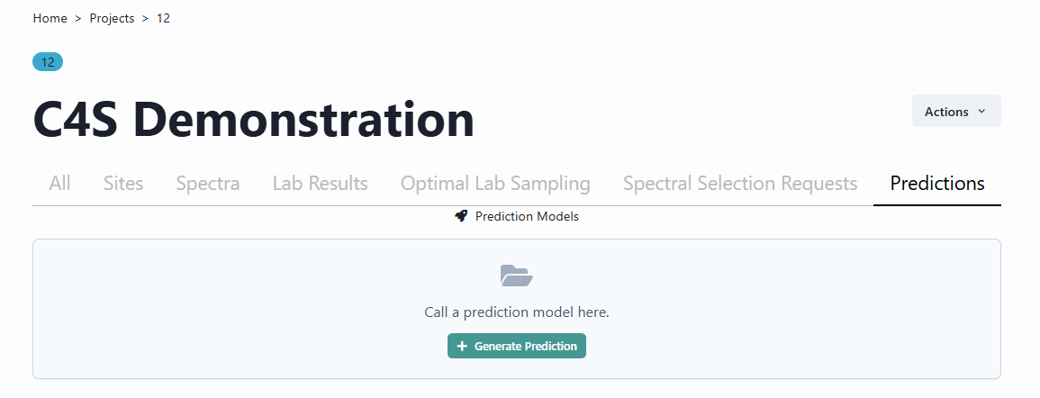
To get started, navigate to the Predictions tab in your Project. From here, click on the ‘Generate Prediction’ icon.
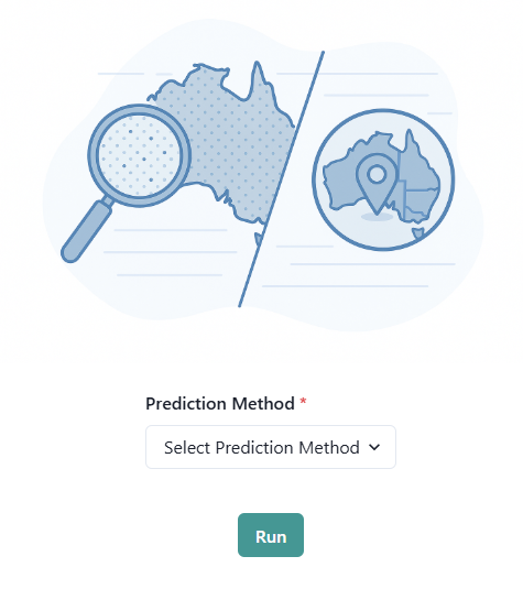
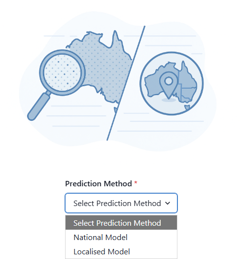
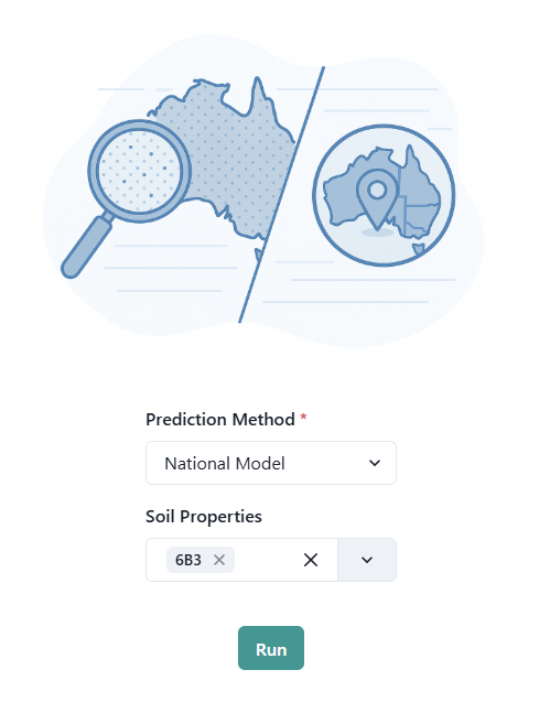
This opens up a new window where the Prediction Method can be selected, the ‘National Model’ or the ‘Localised Model’.
 |
 |
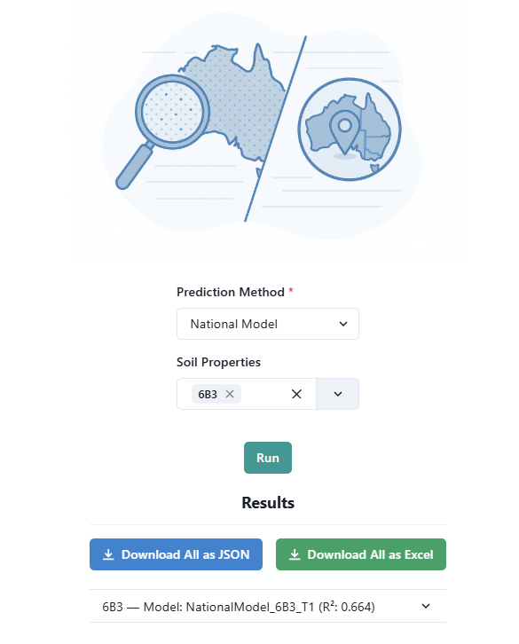
Let’s begin with the selection of a ‘National Model’. In the example below, the prediction of soil organic carbon corresponding to the analytical method 6B3 of dry combustion is chosen (6B3 - Total organic carbon Dumas high-temperature combustion with prior physical removal of charcoal and chemical removal of carbonates). All laboratory method codes listed in the dropdown Menu correspond to the “Green Book” codes (Rayment, G.E. & D.J. Lyons (2011). Soil Chemical Methods - Australasia. CSIRO Publishing). After the user clicked on the Run icon, results from a ‘National Model’ are available and can be downloaded in various file formats.
 |
|

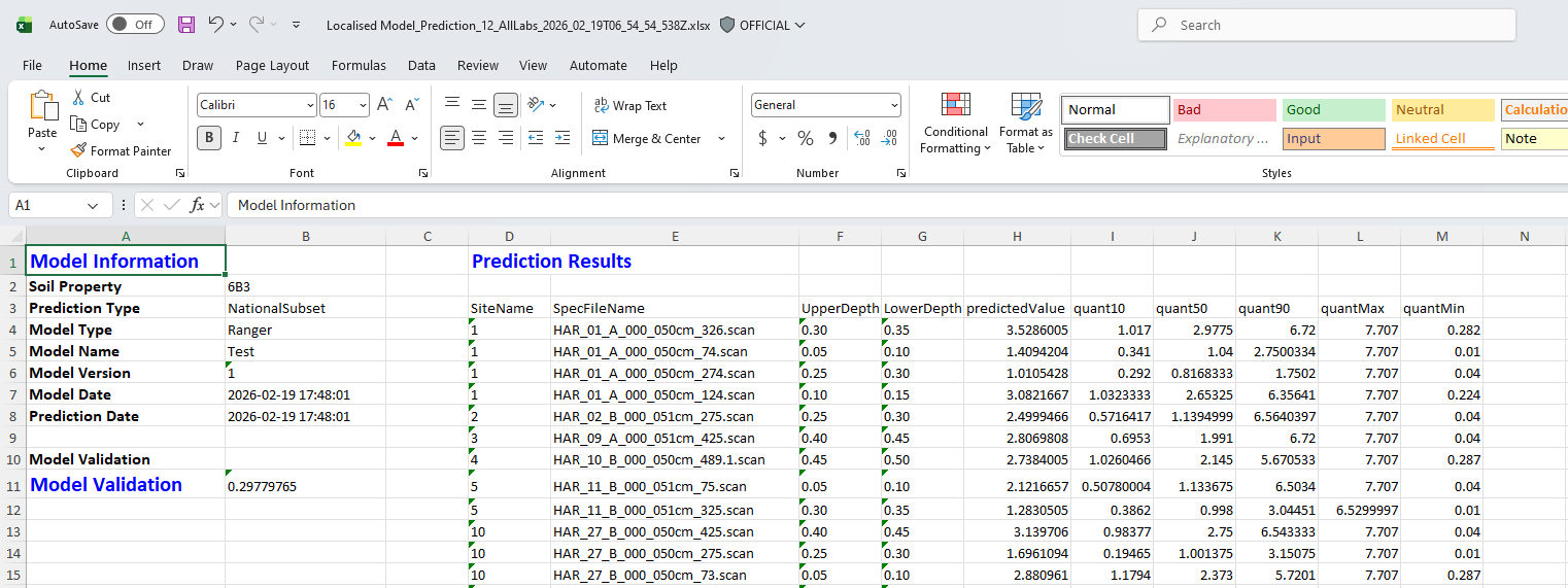
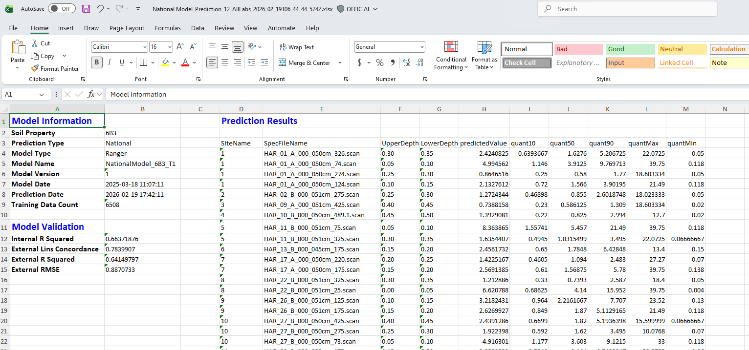
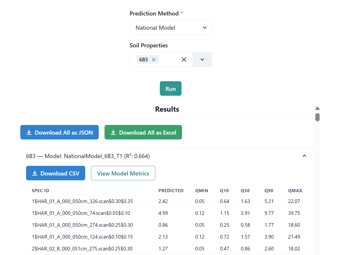
After downloading the Excel format-file, for example, the user can explore the prediction results for soil organic carbon from the ‘National Model’, which also includes the model validation stats for the national model.
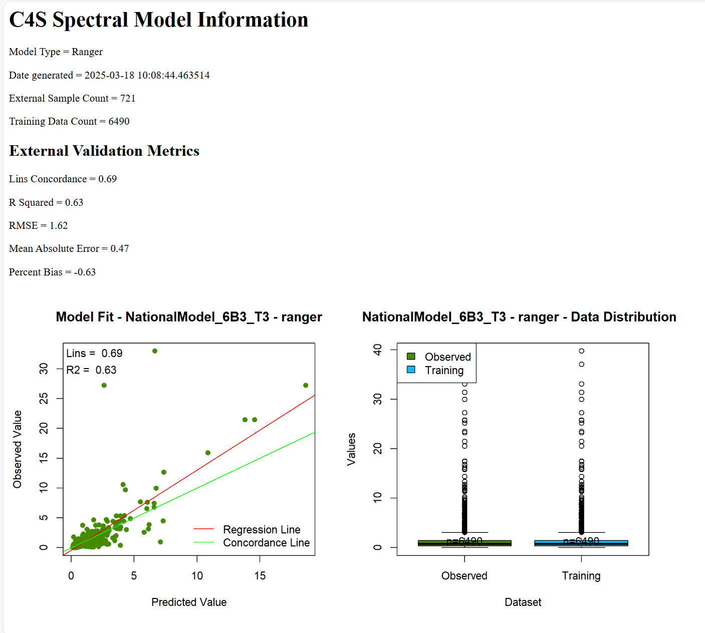
The user can also navigate to the ‘View Model Metrics’ button to look at a visual representation of the statistics of the national model for soil organic carbon.
This is shown below.
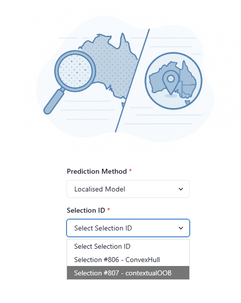
Let’s now select the ‘Localised Model’. In the example below, the selection from the Count of Observations (CoObs) approach or contextualOOB method is chosen. In the ‘Localised Model’, the selection from the national library using the CoObs approach together with your local spectral library is combined, and a hybrid prediction model is created.
 |
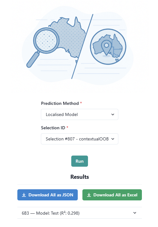 |
Again, after downloading the Excel format-file, for example, the user can explore the prediction results for soil organic carbon from the hybrid ‘Localised Model’, which also includes the model validation stats for the localised model.